Building simulation
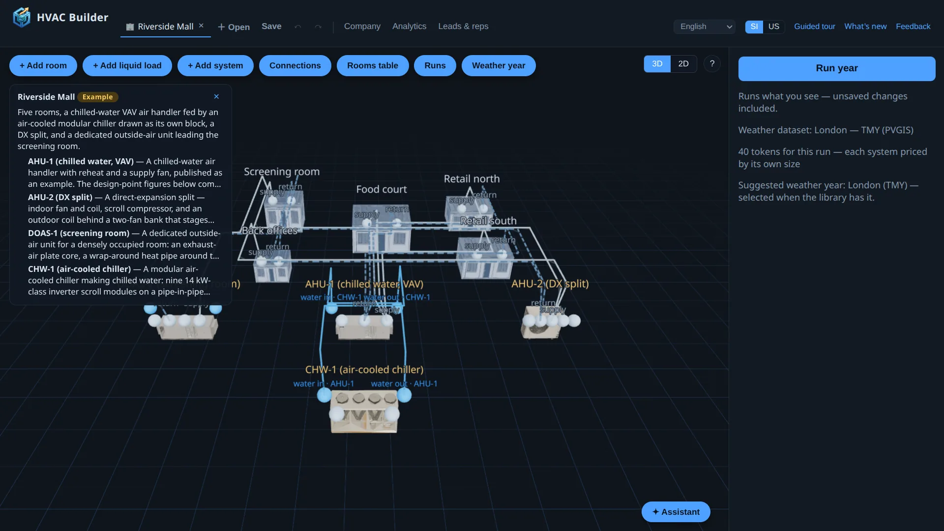
The same building tab scales the analysis from one machine to a whole building. Draw rooms as blocks in a 3D scene and configure each: floor area and height, envelope conductance (UA), day/night internal gains, solar aperture (glazing × SHGC — multiplied by the weather's irradiance), and cooling/heating setpoints. Every field explains itself on hover. A run always executes the draft you see — stored buildings are a convenience, not a prerequisite.
AssignServe each room with one or several machines — your saved systems or published supplier systems, filterable by source; a shared room's load splits equally. Connect them by clicking ports in the scene, like the builder.
ConfigurePer machine: its couplings — every open port of the machine, markable as the supply to the rooms, the return from them (the intake then breathes the rooms' air instead of ambient, while condensers stay on the weather), or a pair with another block's port: a chiller block's water feeding an air handler's coil, an exhaust unit's air feeding a recovery unit, a remote condensing unit's refrigerant feeding an indoor coil (the coil's system declares what arrives on its liquid line under
boundary.refFeeds, the unit's what its suction carries under boundary.refLoads; the pair pins both each hour, and turns round together on a heating hour if the outdoor unit has a reversing valve; a condensing-unit block declared heatRecovery is a three-pipe machine and serves both directions at once, moving the heat through the refrigerant — without it the disagreeing rooms wait). A block that serves water instead of rooms holds a leaving-water setpoint, and a water pair may declare the loop's volume (bufferM3, a buffer tank plus pipework), which the receiving inlet then follows as a first-order lag — the loop's thermal mass. A held outlet may also carry a heating curve (compensation: [[outdoor °C, flow °C], …], read on the outdoor dry bulb, flat past the ends), which is weather compensation — what every hydronic controller draws, and on the apartment example worth 21 % of the year's electricity against holding the cold day's setpoint all year. One water port may carry several pairs to different blocks — a manifold: a chiller's outlet feeding four fan-coil blocks and the outside-air unit, its inlet mixing their returns by flow (the example hotel). An air port is a manifold the same way: several blocks' leaving air into one intake mixes by mass, one outlet feeding several intakes is the same air at each — the building-level twin of several connections on one air port inside a machine. An economiser cannot sit on a manifold leg (its partner runs an hour behind), which is right: the machine ahead is what conditions that air. A machine that serves rooms must declare its supply (supplyAir): the run never detects one. A building may name the TMY city it reads best on (suggestedCity); the building tab selects that year when the building is loaded, fetching it first where the account may — every example declares one, so its published figures come from its own climate. A building may also carry a description — what it is, in a paragraph — shown over the scene when it is loaded, with each machine's own description beneath it; the examples carry their case's tagline. The 3D view is the editor: a machine shows every open port of its graph and a room its supply and return; click one port then another to connect (a machine outlet to a room's supply serves it, a room's return to a machine inlet declares the return, two machines' ports pair them), click a connection and press Delete to remove it, and the Connections list beside the scene shows every one — each is a fact the run reads.RunOne run solves every system against the weather year with full load-following control. Cost: ten times what one solve of that system costs, per simulated year — so 10 tokens for an ordinary machine, and more for a large plant.
ReadPer-room comfort (unmet hours, min/max temperature, 2 °C temperature histograms, month × hour temperature carpets), per-machine sizing analytics (load-duration curves and peak cooling/heating day profiles against delivered capacity), per-system energy, and building totals. Previous building runs reopen from Runs.
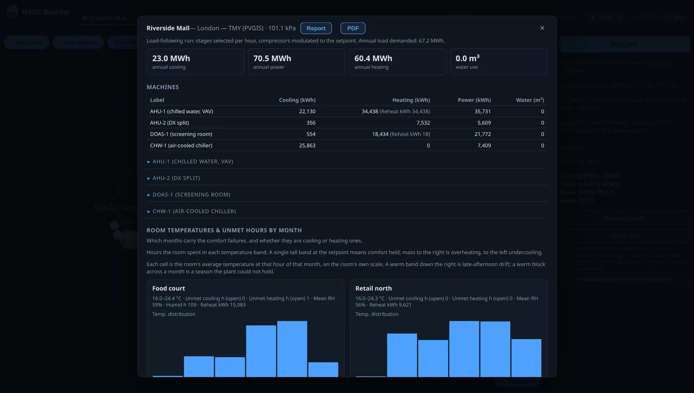
Zone physics is a deliberately transparent 1R1C model: loads from envelope UA + gains against the setpoints, delivered capacity allocated proportionally to demand, and room temperatures that drift toward free-float when a system can't keep up.